Energy scenario design in Aalborg#

Created by Michele Urbani on February 7th, 2025.

The research presented in is replicated here to show how the MOEA package works.

MOEA is based on the PyMOO package for the implementation of the multi-objective evolutionary algorithms (MOEA) and on EnergyPLAN for the energy scenario modeling.

PyMOO breaks down multi-objective optimization into the following steps.

  1. Model description: the optimization models must be encoded in a PyMOO Problem class, or one of its subclasses, e.g., ElementwiseProblem, etc.

    1. The Problem class required to declare a set of high level problem information, such as the number of variables, objective, inequality constraints, and equality constraints.

    2. The objective function evaluation procedure, which in our case calls EnergyPLAN to resolve the instances defined by the solutions found by the algorithm. The output values are then read, and eventually postprocessed, and provided to the algorithm together with constraint violations.

  2. Algorithm declaration: in this case the standard NSGA-II is used.

  3. Resolution: the utility function minimize is used to optimize the problem.

Problem declaration#

The words problem and model are use interchangeably here. In the following, the Aalborg model is explained in details to show an example of problem declarations. To avoid declaring the model twice, the class is declared in moea.models.aalborg.AalborgA and the code is print here with further comments.

import inspect
import numpy as np
import pandas as pd
import matplotlib.pyplot as plt
from IPython.display import display, Markdown

from pymoo.optimize import minimize
from pymoo.indicators.igd import IGD
from pymoo.indicators.hv import Hypervolume

from moea.models import get_model
from moea.algorithms import get_algorithm

Hide code cell output

---------------------------------------------------------------------------
ModuleNotFoundError                       Traceback (most recent call last)
Cell In[1], line 2
      1 import inspect
----> 2 import numpy as np
      3 import pandas as pd
      4 import matplotlib.pyplot as plt

ModuleNotFoundError: No module named 'numpy'
model_name = 'Aalborg'
model = get_model(model_name)

The following cell shows the code used for initializing the model.

The only parameter that can be provided is data_file, i.e., the path to the default EnergyPLAN input data. The default value for this variable is already set to ensure reproducibility of the research.

Input variables are defined as a pandas DataFrame: each row corresponds to a variable, whose index is the variable name in EnergyPLAN, and the columns lb and ub correspond to the lower and upper bound of the variable, respectively.

Later, the parent class is initialized with super().__init__(). This method requires problem infomation, such as the number of variables, the number of (in)equality constraints, the number of objectives, and the upper and lower bounds. Decision variable are assumed to be real numbers.

Even though it is not visible in the code below, the class inherits from the moea.models.base_model.BaseModel class.

# Print models class __init__ code
init_code = inspect.getsource(model.__init__)
display(Markdown("```python\n" + init_code + "```"))
    def __init__(self,
                 data_file: Union[str, Path] = \
                    "Aalborg_2050_Plan_A_44ForOptimization_2objectives.txt",
                 **kwargs):
        """
        Parameters:
        -----------
        - ``data_file``: str or Path

            The path to the input file. This file is used as a template to
            generate the input files for each individual.
            The values will be replaced by the values of the decision variables
            when generating the input files.
        """

        # Define the input variables.
        self.vars = pd.DataFrame.from_dict({
            'input_cap_chp3_el': \
                {'lb':0, 'ub': 1000, "dk0": True, "dk1": False},
            'input_cap_hp3_el': \
                {'lb':0, 'ub': 1000, "dk0": True, "dk1": False},
            'input_cap_pp_el': \
                {'lb': 0, 'ub': 1000, "dk0": None, "dk1": None},
            'input_RES1_capacity': \
                {'lb': 0, 'ub': 1500, "dk0": True, "dk1": False},
            'input_RES2_capacity': \
                {'lb': 0, 'ub': 1500, "dk0": True, "dk1": False},
            'input_RES3_capacity': \
                {'lb': 0, 'ub': 1500, "dk0": True, "dk1": False},
            'input_cap_boiler3_th': \
                {'lb': 0, 'ub': 250, "dk0": None, "dk1": None},
        }, dtype=float, orient='index')

        # Initialize the parent class
        super().__init__(
            n_var=len(self.vars),
            n_ieq_constr=3,
            n_obj=2,
            xl=self.vars['lb'].values,
            xu=self.vars['ub'].values,
            data_file=data_file,
            **kwargs
        )

The evalutation method is the core of the objective function calculation.

The Aalborg model calls EnergyPLAN twice per iterations. During each iteration, the first call to EnergyPLAN sets only the

  • input_cap_chp3_el,

  • input_cap_hp3_el,

  • input_RES1_capacity,

  • input_RES2_capacity,

  • input_RES3_capacity,

variables as input. Then, the annual maximum Boiler 3 Heat and PP Electr. are read from EnergyPLAN results, and they are used to set the value of input_cap_pp_el and input_cap_boiler3_th. Finally, if solutions met certain conditions, EnergyPLAN is called again with the new variable values, and CO2 emissions and cost are used as the objective function values.

The _evaluate method does not return a value but it expects you to set a value for, at the least, the out["F"] value of the out dictionary. This must be a numpy array, whos size is \(N_{solutions} \times N_{objectives}\).

The dictionary values "G" and "H" can be used to declare the left-hand side of inequalities and equalities constraints, respectively. These arrays must have size \(N_{solutoins} \times N_{constraints}\).

eval_code = inspect.getsource(model._evaluate)
display(Markdown("```python\n" + eval_code + "```"))
    def _evaluate(self, x, out, *args, **kwargs):
        self.energyplan.run(
            inputs=[{k: ind[j] for j, k in enumerate(self.vars.index)}
                    for ind in x]
        )

        # Parse the output file
        Y = self.energyplan.read_values(
            "CO2-emission (corrected)",
            "TOTAL ANNUAL COSTS",
            ("Maximum", "import"),
            ("Annual", "heat3- balance"),
            ("Minimum", "stab.- load"),
        )

        # The CO2 emissions are set directly from the results files, whereas
        # the cost is adjusted by the reduction in investment and fixed O&M
        # for the cases where CHP > PP.
        out["F"] = Y[:, :2]

        # CONSTRAINTS
        # Since there are a fes constraints, we evaluate the left-hand side
        # of the constraints and store the values in out["G"].

        # Transmission line capacity of export/import: 160 MW. This constraint
        # enforces the system to produce enough electricity so that it does not
        # require to import more than 160 MW.
        import_constr = np.array(Y[:, 2]) - 160

        # Heat balance. This constraint enforces the system to produce exactly
        # the amount of heat necessary to meet the heat demand.
        heat = - np.array(Y[:, 3])

        # Grid stabilization: More than 30% of power production in all hours
        # must come from units able to supply grid support (see [77] for
        # details on grid stability in EnergyPLAN).
        # This constraint is already taken into account by EnergyPLAN so we
        # just need to subtract the value from 100 to have a constraint that
        # is satisfied when the value is positive.
        stable_load = 100 - np.array(Y[:, 4])

        out["G"] = np.column_stack([
            import_constr,
            stable_load,
            heat,
        ])

Problem resolution#

The utility function minimize is the default way to run an algorithm on a problem of your choice. It requires to pass the model variable, i.e., the variable to which the model has been assigned, the algorithm, and a stopping criterion. Optionally, a seed value can be provided, which enables replicability of results, and verbose can be set to True to visualize runtime infomrmation.

The minimize function returns an objects storing results. Below, we show how to extract some quantities of interest and plot them.

NSGA-2 Algorithm#

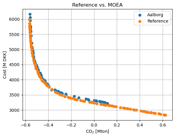
The NSGA-2 algorithm is one of the most popular algorithm for multi-objective optimization and it is used here for benchmarking of results against the Domain Knowledge algorithm proposed by .

model_name = 'Aalborg'
model = get_model(model_name)

algorithm_name = 'NSGA2'
# The population size can be provided when the algorithm is declared
# using the `pop_size` argument. If it is not explicitly set, the
# default value is 100.
algorithm = get_algorithm(algorithm_name)

res = minimize(
    model,
    algorithm,
    ('n_gen', 100),  # The stopping criterion is set to 100 generations
    seed=2903,       # Setting a seed allows us to replicate an experiment
    verbose=True     # Print information while the algorithm is running
)

Hide code cell output

==========================================================================================
n_gen  |  n_eval  | n_nds  |     cv_min    |     cv_avg    |      eps      |   indicator  
==========================================================================================
     1 |      100 |     18 |  0.000000E+00 |  0.3500000000 |             - |             -
     2 |      200 |     26 |  0.000000E+00 |  0.000000E+00 |  0.0084033613 |         ideal
     3 |      300 |     30 |  0.000000E+00 |  0.000000E+00 |  0.0027932961 |         ideal
     4 |      400 |     31 |  0.000000E+00 |  0.000000E+00 |  0.0544822257 |         ideal
     5 |      500 |     34 |  0.000000E+00 |  0.000000E+00 |  0.0076013514 |         ideal
     6 |      600 |     39 |  0.000000E+00 |  0.000000E+00 |  0.0023242142 |             f
     7 |      700 |     41 |  0.000000E+00 |  0.000000E+00 |  0.0050188206 |         ideal
     8 |      800 |     46 |  0.000000E+00 |  0.000000E+00 |  0.0385542169 |         nadir
     9 |      900 |     48 |  0.000000E+00 |  0.000000E+00 |  0.0005496553 |             f
    10 |     1000 |     49 |  0.000000E+00 |  0.000000E+00 |  0.0008170943 |             f
    11 |     1100 |     48 |  0.000000E+00 |  0.000000E+00 |  0.0129119946 |         ideal
    12 |     1200 |     48 |  0.000000E+00 |  0.000000E+00 |  0.0632225434 |         nadir
    13 |     1300 |     47 |  0.000000E+00 |  0.000000E+00 |  0.0003585284 |             f
    14 |     1400 |     46 |  0.000000E+00 |  0.000000E+00 |  0.0006363782 |             f
    15 |     1500 |     48 |  0.000000E+00 |  0.000000E+00 |  0.0040710796 |             f
    16 |     1600 |     46 |  0.000000E+00 |  0.000000E+00 |  0.0009591624 |             f
    17 |     1700 |     43 |  0.000000E+00 |  0.000000E+00 |  0.0024917250 |             f
    18 |     1800 |     45 |  0.000000E+00 |  0.000000E+00 |  0.0038106916 |             f
    19 |     1900 |     50 |  0.000000E+00 |  0.000000E+00 |  0.0014892725 |             f
    20 |     2000 |     48 |  0.000000E+00 |  0.000000E+00 |  0.0050115491 |             f
    21 |     2100 |     45 |  0.000000E+00 |  0.000000E+00 |  0.0021625792 |             f
    22 |     2200 |     45 |  0.000000E+00 |  0.000000E+00 |  0.0024148471 |             f
    23 |     2300 |     47 |  0.000000E+00 |  0.000000E+00 |  0.0026585591 |             f
    24 |     2400 |     47 |  0.000000E+00 |  0.000000E+00 |  0.0011382563 |             f
    25 |     2500 |     47 |  0.000000E+00 |  0.000000E+00 |  0.0013841276 |             f
    26 |     2600 |     48 |  0.000000E+00 |  0.000000E+00 |  0.0027090695 |             f
    27 |     2700 |     49 |  0.000000E+00 |  0.000000E+00 |  0.0003721245 |             f
    28 |     2800 |     45 |  0.000000E+00 |  0.000000E+00 |  0.0031243316 |             f
    29 |     2900 |     43 |  0.000000E+00 |  0.000000E+00 |  0.0011215044 |             f
    30 |     3000 |     46 |  0.000000E+00 |  0.000000E+00 |  0.0032109008 |             f
    31 |     3100 |     39 |  0.000000E+00 |  0.000000E+00 |  0.0008986495 |             f
    32 |     3200 |     41 |  0.000000E+00 |  0.000000E+00 |  0.0039582584 |         ideal
    33 |     3300 |     41 |  0.000000E+00 |  0.000000E+00 |  0.000000E+00 |             f
    34 |     3400 |     43 |  0.000000E+00 |  0.000000E+00 |  0.0014310961 |             f
    35 |     3500 |     44 |  0.000000E+00 |  0.000000E+00 |  0.0162831858 |         nadir
    36 |     3600 |     46 |  0.000000E+00 |  0.000000E+00 |  0.0011649058 |             f
    37 |     3700 |     46 |  0.000000E+00 |  0.000000E+00 |  0.0013589060 |             f
    38 |     3800 |     46 |  0.000000E+00 |  0.000000E+00 |  0.0021869976 |             f
    39 |     3900 |     47 |  0.000000E+00 |  0.000000E+00 |  0.0026560528 |             f
    40 |     4000 |     46 |  0.000000E+00 |  0.000000E+00 |  0.0005291487 |             f
    41 |     4100 |     48 |  0.000000E+00 |  0.000000E+00 |  0.0007449353 |             f
    42 |     4200 |     48 |  0.000000E+00 |  0.000000E+00 |  0.0147270115 |         nadir
    43 |     4300 |     47 |  0.000000E+00 |  0.000000E+00 |  0.0016002111 |             f
    44 |     4400 |     47 |  0.000000E+00 |  0.000000E+00 |  0.0021755776 |             f
    45 |     4500 |     49 |  0.000000E+00 |  0.000000E+00 |  0.0034245738 |             f
    46 |     4600 |     50 |  0.000000E+00 |  0.000000E+00 |  0.1740812379 |         nadir
    47 |     4700 |     51 |  0.000000E+00 |  0.000000E+00 |  0.0007671182 |             f
    48 |     4800 |     53 |  0.000000E+00 |  0.000000E+00 |  0.0021529553 |             f
    49 |     4900 |     56 |  0.000000E+00 |  0.000000E+00 |  0.0035157669 |             f
    50 |     5000 |     59 |  0.000000E+00 |  0.000000E+00 |  0.0217620218 |         ideal
    51 |     5100 |     59 |  0.000000E+00 |  0.000000E+00 |  0.0003559357 |             f
    52 |     5200 |     63 |  0.000000E+00 |  0.000000E+00 |  0.0016965394 |             f
    53 |     5300 |     64 |  0.000000E+00 |  0.000000E+00 |  0.0246490928 |         ideal
    54 |     5400 |     65 |  0.000000E+00 |  0.000000E+00 |  0.0009406508 |             f
    55 |     5500 |     68 |  0.000000E+00 |  0.000000E+00 |  0.0011693682 |             f
    56 |     5600 |     64 |  0.000000E+00 |  0.000000E+00 |  0.0023140777 |             f
    57 |     5700 |     64 |  0.000000E+00 |  0.000000E+00 |  0.0036248207 |             f
    58 |     5800 |     66 |  0.000000E+00 |  0.000000E+00 |  0.0011030939 |             f
    59 |     5900 |     69 |  0.000000E+00 |  0.000000E+00 |  0.0012023392 |             f
    60 |     6000 |     70 |  0.000000E+00 |  0.000000E+00 |  0.0012673768 |             f
    61 |     6100 |     72 |  0.000000E+00 |  0.000000E+00 |  0.0013950530 |             f
    62 |     6200 |     70 |  0.000000E+00 |  0.000000E+00 |  0.0017196931 |             f
    63 |     6300 |     71 |  0.000000E+00 |  0.000000E+00 |  0.0019116433 |             f
    64 |     6400 |     70 |  0.000000E+00 |  0.000000E+00 |  0.0021620285 |             f
    65 |     6500 |     71 |  0.000000E+00 |  0.000000E+00 |  0.0021925879 |             f
    66 |     6600 |     69 |  0.000000E+00 |  0.000000E+00 |  0.0027196743 |             f
    67 |     6700 |     71 |  0.000000E+00 |  0.000000E+00 |  0.0003499835 |             f
    68 |     6800 |     71 |  0.000000E+00 |  0.000000E+00 |  0.0003499835 |             f
    69 |     6900 |     72 |  0.000000E+00 |  0.000000E+00 |  0.0004807693 |             f
    70 |     7000 |     73 |  0.000000E+00 |  0.000000E+00 |  0.0005211733 |             f
    71 |     7100 |     73 |  0.000000E+00 |  0.000000E+00 |  0.0005211733 |             f
    72 |     7200 |     74 |  0.000000E+00 |  0.000000E+00 |  0.0005992580 |             f
    73 |     7300 |     74 |  0.000000E+00 |  0.000000E+00 |  0.0005992580 |             f
    74 |     7400 |     77 |  0.000000E+00 |  0.000000E+00 |  0.0006925613 |             f
    75 |     7500 |     77 |  0.000000E+00 |  0.000000E+00 |  0.0006925613 |             f
    76 |     7600 |     78 |  0.000000E+00 |  0.000000E+00 |  0.0091587517 |         ideal
    77 |     7700 |     79 |  0.000000E+00 |  0.000000E+00 |  0.0001568602 |             f
    78 |     7800 |     79 |  0.000000E+00 |  0.000000E+00 |  0.0001568602 |             f
    79 |     7900 |     79 |  0.000000E+00 |  0.000000E+00 |  0.0001760444 |             f
    80 |     8000 |     79 |  0.000000E+00 |  0.000000E+00 |  0.0001760444 |             f
    81 |     8100 |     80 |  0.000000E+00 |  0.000000E+00 |  0.0005133915 |             f
    82 |     8200 |     81 |  0.000000E+00 |  0.000000E+00 |  0.0007859563 |             f
    83 |     8300 |     77 |  0.000000E+00 |  0.000000E+00 |  0.0011305793 |             f
    84 |     8400 |     78 |  0.000000E+00 |  0.000000E+00 |  0.0012746326 |             f
    85 |     8500 |     79 |  0.000000E+00 |  0.000000E+00 |  0.0012584981 |             f
    86 |     8600 |     80 |  0.000000E+00 |  0.000000E+00 |  0.0014675949 |             f
    87 |     8700 |     80 |  0.000000E+00 |  0.000000E+00 |  0.0014675949 |             f
    88 |     8800 |     79 |  0.000000E+00 |  0.000000E+00 |  0.0015950564 |             f
    89 |     8900 |     80 |  0.000000E+00 |  0.000000E+00 |  0.0016702115 |             f
    90 |     9000 |     84 |  0.000000E+00 |  0.000000E+00 |  0.0021266602 |             f
    91 |     9100 |     84 |  0.000000E+00 |  0.000000E+00 |  0.0021266602 |             f
    92 |     9200 |     85 |  0.000000E+00 |  0.000000E+00 |  0.0022186696 |             f
    93 |     9300 |     85 |  0.000000E+00 |  0.000000E+00 |  0.0022186696 |             f
    94 |     9400 |     85 |  0.000000E+00 |  0.000000E+00 |  0.0022186696 |             f
    95 |     9500 |     88 |  0.000000E+00 |  0.000000E+00 |  0.0025125179 |             f
    96 |     9600 |     88 |  0.000000E+00 |  0.000000E+00 |  0.0001504550 |             f
    97 |     9700 |     87 |  0.000000E+00 |  0.000000E+00 |  0.0004098250 |             f
    98 |     9800 |     89 |  0.000000E+00 |  0.000000E+00 |  0.0005118413 |             f
    99 |     9900 |     89 |  0.000000E+00 |  0.000000E+00 |  0.0005118413 |             f
   100 |    10000 |     86 |  0.000000E+00 |  0.000000E+00 |  0.0007584462 |             f

Results analysis#

# Get the pareto-front
F = res.F

# Load reference data from the paper, no index column and space separated
ref = pd.read_csv('aalborg-reference.csv', sep=' ', header=None,
                  names=['CO2 [Mton]', 'Cost [M DKK]'],
                  index_col=False)

# Plot the pareto-front
plt.scatter(F[:,0], F[:,1], label=model_name)
plt.scatter(ref.values[:,0], ref.values[:,1], label='Reference')
plt.xlabel('CO$_2$ [Mton]')
plt.ylabel('Cost [M DKK]')
plt.title('Reference vs. MOEA')
plt.grid()
plt.legend()

plt.show()
../_images/17369fe5f40f8268b1d59d38554ae3b0bb1dacb3e37419f7cffbb9df040d0f22.png

Convergence analysis#

The results of the paper are used as reference to measure the quality of the solution. We implement the Inverted Generational Distance (IGD) to quantify the distance from any point in the set of solutions \(Z\) to the closest point in the set of reference solutions \(A\).

\[ IGD(A) = \frac{1}{|Z|} \left( \sum_{i=1}^{|Z|} \hat{d}_i ^{\,p} \right) ^{1/p} \]

where \(\hat{d}_i\) represents the Euclidean distance (\(p=2\)) from \(z_i\) to its nearest reference point in \(A\).

The lower the value of the IGD, the closer the set \(A\) to the reference set \(Z\).

igds = {}

ind = IGD(ref.values)
igds[(model_name, algorithm_name)] = ind(res.F)
print("IGD", ind(res.F))
IGD 76.18284671193535

Domain knowledge algorithm#

In , the Domain Knowledge algotithm is proposed to exploit experts’ knowledge of the underlying energy scenario to enhance the MOEA. In the following, the Aalborg model is run using the Domain Knowledge algorithm to check for improvements.

model_name = 'Aalborg'
algorithm_name = 'mahbub2016'

model = get_model(model_name)
algorithm = get_algorithm(algorithm_name, pop_size=100)

res = minimize(
    model,
    algorithm,
    ('n_gen', 100),
    seed=4395,
    verbose=True,
    save_history=True
)

Hide code cell output

==========================================================================================
n_gen  |  n_eval  | n_nds  |     cv_min    |     cv_avg    |      eps      |   indicator  
==========================================================================================
     1 |      101 |     25 |  0.000000E+00 |  0.000000E+00 |             - |             -
     2 |      201 |     32 |  0.000000E+00 |  0.000000E+00 |  0.0033404191 |         ideal
     3 |      301 |     41 |  0.000000E+00 |  0.000000E+00 |  0.0057361377 |         ideal
     4 |      401 |     47 |  0.000000E+00 |  0.000000E+00 |  0.0100558659 |         ideal
     5 |      501 |     55 |  0.000000E+00 |  0.000000E+00 |  0.0058939096 |         nadir
     6 |      601 |     52 |  0.000000E+00 |  0.000000E+00 |  0.0046101364 |             f
     7 |      701 |     52 |  0.000000E+00 |  0.000000E+00 |  0.0044705225 |         ideal
     8 |      801 |     54 |  0.000000E+00 |  0.000000E+00 |  0.0025657139 |             f
     9 |      901 |     65 |  0.000000E+00 |  0.000000E+00 |  0.0144404332 |         nadir
    10 |     1001 |     66 |  0.000000E+00 |  0.000000E+00 |  0.0022245787 |             f
    11 |     1101 |     70 |  0.000000E+00 |  0.000000E+00 |  0.0027536704 |             f
    12 |     1201 |     77 |  0.000000E+00 |  0.000000E+00 |  0.0013924517 |             f
    13 |     1301 |     75 |  0.000000E+00 |  0.000000E+00 |  0.0020051428 |             f
    14 |     1401 |     79 |  0.000000E+00 |  0.000000E+00 |  0.0032309859 |             f
    15 |     1501 |     84 |  0.000000E+00 |  0.000000E+00 |  0.0005660309 |             f
    16 |     1601 |     82 |  0.000000E+00 |  0.000000E+00 |  0.0008093524 |             f
    17 |     1701 |     83 |  0.000000E+00 |  0.000000E+00 |  0.0014721847 |             f
    18 |     1801 |     81 |  0.000000E+00 |  0.000000E+00 |  0.0025234356 |             f
    19 |     1901 |     83 |  0.000000E+00 |  0.000000E+00 |  0.0005034618 |             f
    20 |     2001 |     81 |  0.000000E+00 |  0.000000E+00 |  0.0008049563 |             f
    21 |     2101 |     83 |  0.000000E+00 |  0.000000E+00 |  0.0015762527 |             f
    22 |     2201 |     86 |  0.000000E+00 |  0.000000E+00 |  0.0024739900 |             f
    23 |     2301 |     87 |  0.000000E+00 |  0.000000E+00 |  0.0027360512 |             f
    24 |     2401 |     82 |  0.000000E+00 |  0.000000E+00 |  0.0000545033 |             f
    25 |     2501 |     85 |  0.000000E+00 |  0.000000E+00 |  0.0003818516 |             f
    26 |     2601 |     86 |  0.000000E+00 |  0.000000E+00 |  0.0246478873 |         nadir
    27 |     2701 |     87 |  0.000000E+00 |  0.000000E+00 |  0.0002983740 |             f
    28 |     2801 |     89 |  0.000000E+00 |  0.000000E+00 |  0.0004542409 |             f
    29 |     2901 |     96 |  0.000000E+00 |  0.000000E+00 |  0.0011457728 |             f
    30 |     3001 |     92 |  0.000000E+00 |  0.000000E+00 |  0.0014526398 |             f
    31 |     3101 |     92 |  0.000000E+00 |  0.000000E+00 |  0.1606217617 |         nadir
    32 |     3201 |     97 |  0.000000E+00 |  0.000000E+00 |  0.0007041549 |             f
    33 |     3301 |     99 |  0.000000E+00 |  0.000000E+00 |  0.0010970143 |             f
    34 |     3401 |     91 |  0.000000E+00 |  0.000000E+00 |  0.0013562069 |             f
    35 |     3501 |     85 |  0.000000E+00 |  0.000000E+00 |  0.0016416898 |             f
    36 |     3601 |     90 |  0.000000E+00 |  0.000000E+00 |  0.0018082905 |             f
    37 |     3701 |     93 |  0.000000E+00 |  0.000000E+00 |  0.0021464555 |             f
    38 |     3801 |     94 |  0.000000E+00 |  0.000000E+00 |  0.0026003418 |             f
    39 |     3901 |     96 |  0.000000E+00 |  0.000000E+00 |  0.0061909417 |         nadir
    40 |     4001 |     99 |  0.000000E+00 |  0.000000E+00 |  0.0080801551 |         ideal
    41 |     4101 |     95 |  0.000000E+00 |  0.000000E+00 |  0.0003104271 |             f
    42 |     4201 |     98 |  0.000000E+00 |  0.000000E+00 |  0.0154250082 |         nadir
    43 |     4301 |     98 |  0.000000E+00 |  0.000000E+00 |  0.0001633053 |             f
    44 |     4401 |     97 |  0.000000E+00 |  0.000000E+00 |  0.0006084698 |             f
    45 |     4501 |     96 |  0.000000E+00 |  0.000000E+00 |  0.0011781711 |             f
    46 |     4601 |     98 |  0.000000E+00 |  0.000000E+00 |  0.0014620972 |             f
    47 |     4701 |     94 |  0.000000E+00 |  0.000000E+00 |  0.0016292677 |             f
    48 |     4801 |     98 |  0.000000E+00 |  0.000000E+00 |  0.0022679703 |             f
    49 |     4901 |    100 |  0.000000E+00 |  0.000000E+00 |  0.0055483029 |         nadir
    50 |     5001 |    100 |  0.000000E+00 |  0.000000E+00 |  0.0001971321 |             f
    51 |     5101 |    100 |  0.000000E+00 |  0.000000E+00 |  0.0017860919 |             f
    52 |     5201 |    100 |  0.000000E+00 |  0.000000E+00 |  0.0019824325 |             f
    53 |     5301 |    100 |  0.000000E+00 |  0.000000E+00 |  0.0199733688 |         nadir
    54 |     5401 |    100 |  0.000000E+00 |  0.000000E+00 |  0.0056272757 |         ideal
    55 |     5501 |    100 |  0.000000E+00 |  0.000000E+00 |  0.0002368070 |             f
    56 |     5601 |    100 |  0.000000E+00 |  0.000000E+00 |  0.0003161801 |             f
    57 |     5701 |    100 |  0.000000E+00 |  0.000000E+00 |  0.0005609679 |             f
    58 |     5801 |    100 |  0.000000E+00 |  0.000000E+00 |  0.0007509295 |             f
    59 |     5901 |    100 |  0.000000E+00 |  0.000000E+00 |  0.0010833791 |             f
    60 |     6001 |     99 |  0.000000E+00 |  0.000000E+00 |  0.0011069405 |             f
    61 |     6101 |    100 |  0.000000E+00 |  0.000000E+00 |  0.0014600561 |             f
    62 |     6201 |    100 |  0.000000E+00 |  0.000000E+00 |  0.0016194829 |             f
    63 |     6301 |    100 |  0.000000E+00 |  0.000000E+00 |  0.0016469627 |             f
    64 |     6401 |    100 |  0.000000E+00 |  0.000000E+00 |  0.0016397162 |             f
    65 |     6501 |    100 |  0.000000E+00 |  0.000000E+00 |  0.0018934838 |             f
    66 |     6601 |    100 |  0.000000E+00 |  0.000000E+00 |  0.0018934838 |             f
    67 |     6701 |    100 |  0.000000E+00 |  0.000000E+00 |  0.0018162553 |             f
    68 |     6801 |    100 |  0.000000E+00 |  0.000000E+00 |  0.0018162553 |             f
    69 |     6901 |    100 |  0.000000E+00 |  0.000000E+00 |  0.0018348641 |             f
    70 |     7001 |     99 |  0.000000E+00 |  0.000000E+00 |  0.0020139563 |             f
    71 |     7101 |     99 |  0.000000E+00 |  0.000000E+00 |  0.0022637948 |             f
    72 |     7201 |    100 |  0.000000E+00 |  0.000000E+00 |  0.0025541812 |             f
    73 |     7301 |    100 |  0.000000E+00 |  0.000000E+00 |  0.0000373922 |             f
    74 |     7401 |    100 |  0.000000E+00 |  0.000000E+00 |  0.0001506969 |             f
    75 |     7501 |    100 |  0.000000E+00 |  0.000000E+00 |  0.0001506969 |             f
    76 |     7601 |    100 |  0.000000E+00 |  0.000000E+00 |  0.0002110996 |             f
    77 |     7701 |    100 |  0.000000E+00 |  0.000000E+00 |  0.0003455002 |             f
    78 |     7801 |    100 |  0.000000E+00 |  0.000000E+00 |  0.0004560361 |             f
    79 |     7901 |    100 |  0.000000E+00 |  0.000000E+00 |  0.0009939226 |             f
    80 |     8001 |    100 |  0.000000E+00 |  0.000000E+00 |  0.0009939226 |             f
    81 |     8101 |    100 |  0.000000E+00 |  0.000000E+00 |  0.0010535633 |             f
    82 |     8201 |    100 |  0.000000E+00 |  0.000000E+00 |  0.0010535633 |             f
    83 |     8301 |    100 |  0.000000E+00 |  0.000000E+00 |  0.0014900741 |             f
    84 |     8401 |    100 |  0.000000E+00 |  0.000000E+00 |  0.0016099834 |             f
    85 |     8501 |    100 |  0.000000E+00 |  0.000000E+00 |  0.0016415950 |             f
    86 |     8601 |    100 |  0.000000E+00 |  0.000000E+00 |  0.0016634530 |             f
    87 |     8701 |    100 |  0.000000E+00 |  0.000000E+00 |  0.0016951345 |             f
    88 |     8801 |    100 |  0.000000E+00 |  0.000000E+00 |  0.0016951345 |             f
    89 |     8901 |    100 |  0.000000E+00 |  0.000000E+00 |  0.0017488062 |             f
    90 |     9001 |    100 |  0.000000E+00 |  0.000000E+00 |  0.0018219614 |             f
    91 |     9101 |     99 |  0.000000E+00 |  0.000000E+00 |  0.0020389221 |             f
    92 |     9201 |    100 |  0.000000E+00 |  0.000000E+00 |  0.0020925876 |             f
    93 |     9301 |    100 |  0.000000E+00 |  0.000000E+00 |  0.0023591410 |             f
    94 |     9401 |    100 |  0.000000E+00 |  0.000000E+00 |  0.0025183852 |             f
    95 |     9501 |    100 |  0.000000E+00 |  0.000000E+00 |  0.000000E+00 |             f
    96 |     9601 |    100 |  0.000000E+00 |  0.000000E+00 |  0.0002535470 |             f
    97 |     9701 |    100 |  0.000000E+00 |  0.000000E+00 |  0.0002909391 |             f
    98 |     9801 |    100 |  0.000000E+00 |  0.000000E+00 |  0.0003685971 |             f
    99 |     9901 |    100 |  0.000000E+00 |  0.000000E+00 |  0.0003933462 |             f
   100 |    10001 |    100 |  0.000000E+00 |  0.000000E+00 |  0.0005151303 |             f
# Get the pareto-front
F = res.F

# Load reference data from the paper, no index column and space separated
ref = pd.read_csv('aalborg-reference.csv', sep=' ', header=None,
                  names=['CO2 [Mton]', 'Cost [M DKK]'],
                  index_col=False)

# Plot the pareto-front
plt.scatter(F[:,0], F[:,1], label=model_name)
plt.scatter(ref.values[:,0], ref.values[:,1], label='Reference')
plt.xlabel('CO$_2$ [Mton]')
plt.ylabel('Cost [M DKK]')
plt.title('Reference vs. MOEA')
plt.grid()
plt.legend()

plt.show()
../_images/ed1d4c6f7a73d42a27301d9c366ad6f2171bbab2de5b0c56f6a2205d4d575abb.png

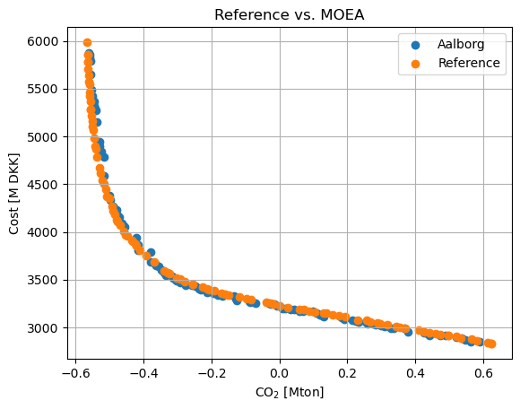
Since the Pareto front from the paper is available, we use is to calculate the inverted generational distance (IGD) to the front obtained by the domain knowledge algorithm.

ind = IGD(ref.values)
print("IGD", ind(res.F))
IGD 15.60073096498567

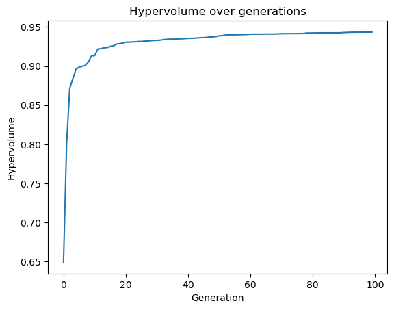
To furhter show that the algorithm converged to a stable front, the hyper- volume (HV) measure is used. HV values are normalized to be independent of problem values and focus on the convergence of results. It is worth mentioning that convergence is tested to the stability of HV values with the number of generations, and it should asymptotically tend to a value. It does not matter that this value is lower than one.

# Calculate the reference point
ref_point = np.max(np.vstack([i.pop.get("F") for i in res.history]), axis=0)
# Extract the fronts from the history
fronts = [i.opt.get("F") for i in res.history]
# Normalize the fronts
normalized_fronts = [i / ref_point for i in fronts]
# Initialize the hypervolume indicator with the reference point (1, 1)
hv = Hypervolume(np.array([1, 1]))
# Calculate the hypervolume for each front
hv_vals = [hv(f) for f in normalized_fronts]

# Plot the hypervolume over generations
plt.plot(hv_vals)
plt.xlabel("Generation")
plt.ylabel("Hypervolume")
plt.title("Hypervolume over generations")
plt.show()
../_images/d0371b9b80f218fd9d41f1ed7fabc40399ee9d804c86eb07268bf4a6d2d9fd77.png

References#