Optimized energy scenarios Giudicarie Esteriori
Created by Michele Urbani.
In this notebook, we replicate the study in .
Problem description
Decision variables
The decision variables are:
PV capacity: the amount of installed PV capacity is 5 MW and it is
as the lower bound for the variable, whereas the calculated maximum PV capacity
is 42 MW, which is the upper bound.
Heat production technologies: individual wood, oil, LPG boilers, and
gound source heat pumps are decision variables expressed as percentages of the
total.
Wood organic ranking cycle micro cogeneration provides both thermal and
electrical power
Constraints
The are two constraints: the first concerns the variables at points 2 and 3 of
the list above, which must sum to 1. The second constraints limits the total
wood consumption to be less than 57 GWh/year.
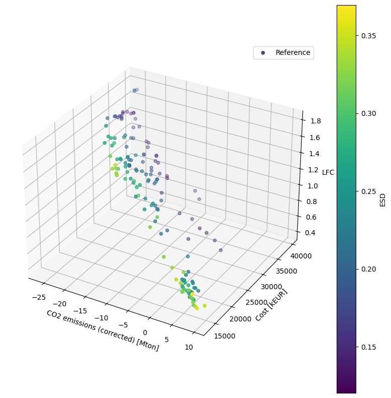
Optimization objectives
There are four optimization objectives.
CO\(_2\) minimization: the value of produced CO\(_2\) is
CO2-emission (corrected) in EnergyPLAN output.
Annual cost minimization: the annual cost is the sum of the annual
investment cost, variable operational and maintenance (O&M) cost, fixed
operational and maintenacne cost, and the variable O&M and fixed O&M costs.
Load following capacity (LFC) minimization: the LFC expresses how much
electricity production follows electrivity demand over a period (yearly in this
case).
Energy system dependency (ESD) minimization concerns the reduction of
foreign energy import.
Problem declaration
The _evaluate method is analyzed in the following.
2025-08-05 11:30:46.109 | INFO | moea.config:<module>:11 - PROJ_ROOT path is: C:\Users\murbani\moea
Show code cell output
Hide code cell output
==========================================================================================
n_gen  |  n_eval  | n_nds  |     cv_min    |     cv_avg    |      eps      |   indicator
==========================================================================================
     1 |      100 |      3 |  0.000000E+00 |  2.858730E+01 |             - |             -
     2 |      200 |      4 |  0.000000E+00 |  1.649660E+01 |  0.3552624049 |         ideal
     3 |      300 |      9 |  0.000000E+00 |  1.146360E+01 |  0.0961991400 |         ideal
     4 |      400 |     12 |  0.000000E+00 |  8.1340000000 |  0.0484775694 |             f
     5 |      500 |     16 |  0.000000E+00 |  6.3120000000 |  0.0890224284 |             f
     6 |      600 |     20 |  0.000000E+00 |  4.9813000000 |  0.0483322873 |             f
     7 |      700 |     22 |  0.000000E+00 |  3.5060000000 |  0.0378091828 |             f
     8 |      800 |     25 |  0.000000E+00 |  2.1549000000 |  0.0384412607 |             f
     9 |      900 |     29 |  0.000000E+00 |  1.3603000000 |  0.1375484273 |         ideal
    10 |     1000 |     32 |  0.000000E+00 |  0.7752000000 |  0.1191417999 |         nadir
    11 |     1100 |     37 |  0.000000E+00 |  0.2903000000 |  0.0293129477 |         ideal
    12 |     1200 |     33 |  0.000000E+00 |  0.000000E+00 |  0.0177090025 |         ideal
    13 |     1300 |     37 |  0.000000E+00 |  0.000000E+00 |  0.0783561236 |         ideal
    14 |     1400 |     40 |  0.000000E+00 |  0.000000E+00 |  0.0112778117 |             f
    15 |     1500 |     38 |  0.000000E+00 |  0.000000E+00 |  0.0291398458 |         ideal
    16 |     1600 |     43 |  0.000000E+00 |  0.000000E+00 |  0.0190765816 |             f
    17 |     1700 |     48 |  0.000000E+00 |  0.000000E+00 |  0.0436931819 |         ideal
    18 |     1800 |     55 |  0.000000E+00 |  0.000000E+00 |  0.0153563429 |             f
    19 |     1900 |     56 |  0.000000E+00 |  0.000000E+00 |  0.0022993929 |             f
    20 |     2000 |     57 |  0.000000E+00 |  0.000000E+00 |  0.0739566735 |         nadir
    21 |     2100 |     58 |  0.000000E+00 |  0.000000E+00 |  0.0018151609 |             f
    22 |     2200 |     54 |  0.000000E+00 |  0.000000E+00 |  0.1415977096 |         ideal
    23 |     2300 |     54 |  0.000000E+00 |  0.000000E+00 |  0.0043143086 |             f
    24 |     2400 |     57 |  0.000000E+00 |  0.000000E+00 |  0.1269304366 |         nadir
    25 |     2500 |     62 |  0.000000E+00 |  0.000000E+00 |  0.0066303390 |         ideal
    26 |     2600 |     63 |  0.000000E+00 |  0.000000E+00 |  0.0635244915 |         ideal
    27 |     2700 |     66 |  0.000000E+00 |  0.000000E+00 |  0.0065035809 |             f
    28 |     2800 |     66 |  0.000000E+00 |  0.000000E+00 |  0.0032630202 |             f
    29 |     2900 |     68 |  0.000000E+00 |  0.000000E+00 |  0.0828845031 |         nadir
    30 |     3000 |     68 |  0.000000E+00 |  0.000000E+00 |  0.0121824457 |         nadir
    31 |     3100 |     72 |  0.000000E+00 |  0.000000E+00 |  0.0063933243 |             f
    32 |     3200 |     74 |  0.000000E+00 |  0.000000E+00 |  0.0338385111 |         ideal
    33 |     3300 |     76 |  0.000000E+00 |  0.000000E+00 |  0.0030370655 |             f
    34 |     3400 |     80 |  0.000000E+00 |  0.000000E+00 |  0.0936090494 |         nadir
    35 |     3500 |     82 |  0.000000E+00 |  0.000000E+00 |  0.0018662569 |             f
    36 |     3600 |     85 |  0.000000E+00 |  0.000000E+00 |  0.0215401698 |         nadir
    37 |     3700 |     88 |  0.000000E+00 |  0.000000E+00 |  0.0030154604 |             f
    38 |     3800 |     91 |  0.000000E+00 |  0.000000E+00 |  0.0014404805 |             f
    39 |     3900 |     91 |  0.000000E+00 |  0.000000E+00 |  0.0014404805 |             f
    40 |     4000 |     92 |  0.000000E+00 |  0.000000E+00 |  0.0022239877 |             f
    41 |     4100 |     92 |  0.000000E+00 |  0.000000E+00 |  0.0030115693 |             f
    42 |     4200 |     93 |  0.000000E+00 |  0.000000E+00 |  0.0001717173 |             f
    43 |     4300 |     94 |  0.000000E+00 |  0.000000E+00 |  0.0289100189 |         ideal
    44 |     4400 |     97 |  0.000000E+00 |  0.000000E+00 |  0.0068740453 |         ideal
    45 |     4500 |     98 |  0.000000E+00 |  0.000000E+00 |  0.0005355608 |             f
    46 |     4600 |     98 |  0.000000E+00 |  0.000000E+00 |  0.0005355608 |             f
    47 |     4700 |    100 |  0.000000E+00 |  0.000000E+00 |  0.0019075056 |             f
    48 |     4800 |    100 |  0.000000E+00 |  0.000000E+00 |  0.0034581768 |             f
    49 |     4900 |    100 |  0.000000E+00 |  0.000000E+00 |  0.0007732338 |             f
    50 |     5000 |    100 |  0.000000E+00 |  0.000000E+00 |  0.0024444155 |             f
    51 |     5100 |    100 |  0.000000E+00 |  0.000000E+00 |  0.0042405858 |             f
    52 |     5200 |    100 |  0.000000E+00 |  0.000000E+00 |  0.0009037632 |             f
    53 |     5300 |    100 |  0.000000E+00 |  0.000000E+00 |  0.0009037632 |             f
    54 |     5400 |    100 |  0.000000E+00 |  0.000000E+00 |  0.0047300319 |             f
    55 |     5500 |    100 |  0.000000E+00 |  0.000000E+00 |  0.0005427791 |             f
    56 |     5600 |    100 |  0.000000E+00 |  0.000000E+00 |  0.0013624404 |             f
    57 |     5700 |    100 |  0.000000E+00 |  0.000000E+00 |  0.0026811135 |             f
    58 |     5800 |    100 |  0.000000E+00 |  0.000000E+00 |  0.0007947801 |             f
    59 |     5900 |    100 |  0.000000E+00 |  0.000000E+00 |  0.0007947801 |             f
    60 |     6000 |    100 |  0.000000E+00 |  0.000000E+00 |  0.0046588147 |             f
    61 |     6100 |    100 |  0.000000E+00 |  0.000000E+00 |  0.0015234393 |             f
    62 |     6200 |    100 |  0.000000E+00 |  0.000000E+00 |  0.0060813605 |         ideal
    63 |     6300 |    100 |  0.000000E+00 |  0.000000E+00 |  0.0017661701 |             f
    64 |     6400 |    100 |  0.000000E+00 |  0.000000E+00 |  0.0017661701 |             f
    65 |     6500 |    100 |  0.000000E+00 |  0.000000E+00 |  0.0025688800 |             f
    66 |     6600 |    100 |  0.000000E+00 |  0.000000E+00 |  0.000000E+00 |             f
    67 |     6700 |    100 |  0.000000E+00 |  0.000000E+00 |  0.000000E+00 |             f
    68 |     6800 |    100 |  0.000000E+00 |  0.000000E+00 |  0.0005073179 |             f
    69 |     6900 |    100 |  0.000000E+00 |  0.000000E+00 |  0.0005073179 |             f
    70 |     7000 |    100 |  0.000000E+00 |  0.000000E+00 |  0.0012420452 |             f
    71 |     7100 |    100 |  0.000000E+00 |  0.000000E+00 |  0.0022084658 |             f
    72 |     7200 |    100 |  0.000000E+00 |  0.000000E+00 |  0.0034385588 |             f
    73 |     7300 |    100 |  0.000000E+00 |  0.000000E+00 |  0.000000E+00 |             f
    74 |     7400 |    100 |  0.000000E+00 |  0.000000E+00 |  0.0005617363 |             f
    75 |     7500 |    100 |  0.000000E+00 |  0.000000E+00 |  0.0006890537 |             f
    76 |     7600 |    100 |  0.000000E+00 |  0.000000E+00 |  0.0006890537 |             f
    77 |     7700 |    100 |  0.000000E+00 |  0.000000E+00 |  0.0006890537 |             f
    78 |     7800 |     99 |  0.000000E+00 |  0.000000E+00 |  0.0028546566 |             f
    79 |     7900 |    100 |  0.000000E+00 |  0.000000E+00 |  0.0179338561 |         ideal
    80 |     8000 |    100 |  0.000000E+00 |  0.000000E+00 |  0.0004894304 |             f
    81 |     8100 |    100 |  0.000000E+00 |  0.000000E+00 |  0.0012335465 |             f
    82 |     8200 |    100 |  0.000000E+00 |  0.000000E+00 |  0.0031946710 |         ideal
    83 |     8300 |    100 |  0.000000E+00 |  0.000000E+00 |  0.0003906560 |             f
    84 |     8400 |    100 |  0.000000E+00 |  0.000000E+00 |  0.0003906560 |             f
    85 |     8500 |    100 |  0.000000E+00 |  0.000000E+00 |  0.0010319648 |             f
    86 |     8600 |    100 |  0.000000E+00 |  0.000000E+00 |  0.0010319648 |             f
    87 |     8700 |    100 |  0.000000E+00 |  0.000000E+00 |  0.0010319648 |             f
    88 |     8800 |     99 |  0.000000E+00 |  0.000000E+00 |  0.0015746528 |             f
    89 |     8900 |     99 |  0.000000E+00 |  0.000000E+00 |  0.0020728633 |             f
    90 |     9000 |    100 |  0.000000E+00 |  0.000000E+00 |  0.0028910149 |             f
    91 |     9100 |    100 |  0.000000E+00 |  0.000000E+00 |  0.0007011033 |             f
    92 |     9200 |    100 |  0.000000E+00 |  0.000000E+00 |  0.0010852210 |             f
    93 |     9300 |    100 |  0.000000E+00 |  0.000000E+00 |  0.0010852210 |             f
    94 |     9400 |    100 |  0.000000E+00 |  0.000000E+00 |  0.0010852210 |             f
    95 |     9500 |    100 |  0.000000E+00 |  0.000000E+00 |  0.0010852210 |             f
    96 |     9600 |    100 |  0.000000E+00 |  0.000000E+00 |  0.0010852210 |             f
    97 |     9700 |    100 |  0.000000E+00 |  0.000000E+00 |  0.0010852210 |             f
    98 |     9800 |    100 |  0.000000E+00 |  0.000000E+00 |  0.0020574463 |             f
    99 |     9900 |    100 |  0.000000E+00 |  0.000000E+00 |  0.0026504594 |             f
   100 |    10000 |    100 |  0.000000E+00 |  0.000000E+00 |  0.0004154629 |             f
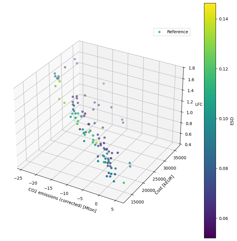
Results analysis
Convergence analysis
The results of the paper are used as reference to
measure the quality of the solution. We implement the Inverted Generational
Distance (IGD) to quantify the distance from any
point in the set of solutions \(Z\) to the closest point in the set of
reference solutions \(A\).
\[
IGD(A) = \frac{1}{|Z|} \left( \sum_{i=1}^{|Z|} \hat{d}_i ^{\,p} \right) ^{1/p}
\]
where \(\hat{d}_i\) represents the Euclidean distance (\(p=2\)) from \(z_i\) to its
nearest reference point in \(A\).
The lower the value of the IGD, the closer the set \(A\) to the reference set
\(Z\).